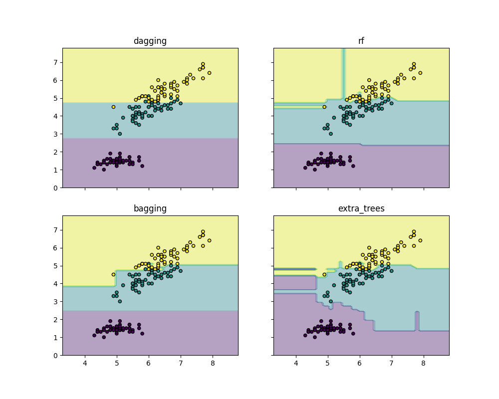
Dagging Decision Regions

In this plot we can compare the decision regions of a dagging model on iris dataset against Random Forest, Bagging and Extra Trees.

print(__doc__)

from itertools import product

import numpy as np
import matplotlib.pyplot as plt

import dagging
from sklearn import datasets
from sklearn.ensemble import (
    BaggingClassifier,
    RandomForestClassifier,
    ExtraTreesClassifier,
)

# Loading some example data
iris = datasets.load_iris()
X = iris.data[:, [0, 2]]
y = iris.target

# Training classifiers
estimators = dict(
    dagging=dagging.DaggingClassifier(random_state=0, n_estimators=10),
    rf=RandomForestClassifier(random_state=0, n_estimators=10),
    bagging=BaggingClassifier(random_state=0, n_estimators=10),
    extra_trees=ExtraTreesClassifier(random_state=0, n_estimators=10),
)

for estimator in estimators.values():
    estimator.fit(X, y)

# Plotting decision regions
x_min, x_max = X[:, 0].min() - 1, X[:, 0].max() + 1
y_min, y_max = X[:, 1].min() - 1, X[:, 1].max() + 1
xx, yy = np.meshgrid(np.arange(x_min, x_max, 0.1), np.arange(y_min, y_max, 0.1))

f, axarr = plt.subplots(2, 2, sharex="col", sharey="row", figsize=(10, 8))

for idx, clf, tt in zip(
    product([0, 1], [0, 1]),
    [e for e in estimators.values()],
    [name for name in estimators.keys()],
):

    Z = clf.predict(np.c_[xx.ravel(), yy.ravel()])
    Z = Z.reshape(xx.shape)

    axarr[idx[0], idx[1]].contourf(xx, yy, Z, alpha=0.4)
    axarr[idx[0], idx[1]].scatter(X[:, 0], X[:, 1], c=y, s=20, edgecolor="k")
    axarr[idx[0], idx[1]].set_title(tt)

plt.show()